Images and Pixels
|
This tutorial is for Processing's Python Mode. If you see any errors or have comments, please let us know. This tutorial is adapted from the book, Learning Processing, by Daniel Shiffman, published by Morgan Kaufmann Publishers, Copyright © 2008 Elsevier Inc. All rights reserved.
A digital image is nothing more than data -- numbers indicating variations of red, green, and blue at a particular location on a grid of pixels. Most of the time, we view these pixels as miniature rectangles sandwiched together on a computer screen. With a little creative thinking and some lower level manipulation of pixels with code, however, we can display that information in a myriad of ways. This tutorial is dedicated to breaking out of simple shape drawing in Processing and using images (and their pixels) as the building blocks of Processing graphics. Getting started with images.
Hopefully, you are comfortable with the idea of data types. You probably specify them often -- a float variable "speed", an int "x", etc. These are all primitive data types, bits sitting in the computer's memory ready for our use. Though perhaps a bit trickier, you hopefully also use objects, complex data types that store multiple pieces of data (along with functionality) -- a "Ball" class, for example, might include floating point variables for location, size, and speed as well as methods to move, display itself, and so on.
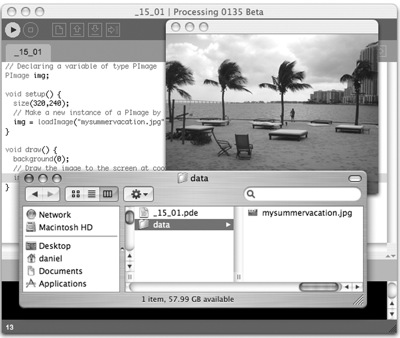
def setup():
  global img
  size(320,240)
  # Make a new instance of a PImage by loading an image file
  # Declaring a variable of type PImage
  img = loadImage("mysummervacation.jpg")

def draw():
  global img
  background(0);
  # Draw the image to the screen at coordinate (0,0)
  image(img,0,0)
Using an instance of a PImage object is no different than using a user-defined class.
We declare a variable img and assign a newly created instance of the PImage class to it by calling the . loadImage() takes one argument, a String indicating a file name, and loads the that file into memory. loadImage() looks for image files stored in your Processing sketch's "data" folder.
 In the above example, it may seem a bit peculiar that we never called a "constructor" to instantiate the PImage object, saying "PImage()". After all, in most object-related examples, a constructor is a must for producing an object instance. mySpaceship = Spaceship(); myFlower = Flower(25);
img = loadImage("file.jpg");
In fact, the loadImage() function performs the work of a constructor, returning a brand new instance of a PImage object generated from the specified filename. We can think of it as the PImage constructor for loading images from a file. For creating a blank image, the createImage() function is used.
# Create a blank image, 200x200 pixels with RGB color
img = createImage(200,200,RGB)
image(img,10,20,90,60) Your very first image processing filter
When displaying an image, you might like to alter its appearance. Perhaps you would like the image to appear darker, transparent, blue-ish, etc. This type of simple image filtering is achieved with Processing's tint() function. tint() is essentially the image equivalent of shape's fill(), setting the color and alpha transparency for displaying an image on screen. An image, nevertheless, is not usually all one color. The arguments for tint() simply specify how much of a given color to use for every pixel of that image, as well as how transparent those pixels should appear.
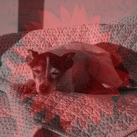
sunflower = loadImage("sunflower.jpg")
dog = loadImage("dog.jpg")
background(dog)
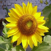
# The image retains its original state. tint(255) image(sunflower,0,0) 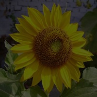 # The image appears darker. tint(100) image(sunflower,0,0)
 # The image is at 50% opacity. tint(255,127) image(sunflower,0,0)
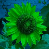
# None of its red, most of its green, and all of its blue.
tint(0,200,255)
image(sunflower,0,0)
# The image is tinted red and transparent.
tint(255,0,0,100)
image(sunflower,0,0)
Pixels, pixels, and more pixels
If you've just begun using Processing you may have mistakenly thought that the only offered means for drawing to the screen is through a function call. "Draw a line between these points" or "Fill an ellipse with red" or "load this JPG image and place it on the screen here." But somewhere, somehow, someone had to write code that translates these function calls into setting the individual pixels on the screen to reflect the requested shape. A line doesn't appear because we say line(), it appears because we color all the pixels along a linear path between two points. Fortunately, we don't have to manage this lower-level-pixel-setting on a day-to-day basis. We have the developers of Processing (and Java) to thank for the many drawing functions that take care of this business.
def setup():
    size(200, 200)
    # Before we deal with pixels
    loadPixels()
    changePixels()

def changePixels():
    # Loop through every pixel
    for i in xrange(len(pixels)):
        # Pick a random number, 0 to 255
        rand = random(255)
        # Create a grayscale color based on random number
        c = color(rand)
        # Set pixel at that location to random color
        pixels[i] = c

    # When we are finished dealing with pixels
    updatePixels()
In the above example, because the colors are set randomly, we didn't have to worry about where the pixels are onscreen as we access them, since we are simply setting all the pixels with no regard to their relative location. However, in many image processing applications, the XY location of the pixels themselves is crucial information. A simple example of this might be, set every even column of pixels to white and every odd to black. How could you do this with a one dimensional pixel array? How do you know what column or row any given pixel is in?
Example: Setting Pixels according to their 2D location
def setup():
    size(200,200)
    loadPixels()
    changePixels()

def changePixels():
    # Loop through every pixel column
    for x in xrange(width):
        # Loop through every pixel row
        for y in xrange(height):
            # Use the formula to find the 1D location
            loc = x + y * width;
            if (x % 2 == 0): # If we are an even column
                pixels[loc] = color(255)
            else:            # If we are an odd column
                pixels[loc] = color(0)

    updatePixels()
Intro To Image Processing
The previous section looked at examples that set pixel values according to an arbitrary calculation. We will now look at how we might set pixels according those found in an existing PImage object. Here is some pseudo-code.
img = createImage(320,240,RGB) # Make a PImage object
print(img.width)  # Yields 320
print(img.height) # Yields 240
img.pixels[0] = color(255,0,0)  # Sets the first pixel of the image to red
# Display a 200x200 pixel image, pixel by pixel.
def setup():
    global img
    size(200, 200)
    img = loadImage("sunflower.jpg")

def draw():
    loadPixels()
    # Since we are going to access the image's pixels too
    img.loadPixels()
    for y in xrange(height):
        for x in xrange(width):
            loc = x + y*width

            # The functions red(), green(), and blue() pull out the
            # 3 color components from a pixel.
            r = red(img.pixels[loc])
            g = green(img.pixels[loc])
            b = blue(img.pixels[loc])

            # Image Processing would go here
            # If we were to change the RGB values, we would do it here,
            # before setting the pixel in the display window.

            # Set the display pixel to the image pixel
            pixels[loc] =  color(r,g,b)

    updatePixels()
imageLoc = x + y*img.width

displayLoc = x + y*width
Our second image filter, making our own "tint"
Just a few paragraphs ago, we were enjoying a relaxing coding session, colorizing images and adding alpha transparency with the friendly tint()method. For basic filtering, this method did the trick. The pixel by pixel method, however, will allow us to develop custom algorithms for mathematically altering the colors of an image. Consider brightness -- brighter colors have higher values for their red, green, and blue components. It follows naturally that we can alter the brightness of an image by increasing or decreasing the color components of each pixel. In the next example, we dynamically increase or decrease those values based on the mouse's horizontal location. (Note, the next two examples include only the image processing loop itself, the rest of the code is assumed.)
for x in xrange(img.width):
    for y in xrange(img.height):
        # Calculate the 1D pixel location
        loc = x + y*img.width
        # Get the R,G,B values from image
        r = red(img.pixels[loc])
        g = green(img.pixels[loc])
        b = blue(img.pixels[loc])

        # Change brightness according to the mouse here
        adjustBrightness = (float(mouseX) / width) * 8.0
        r *= adjustBrightness
        g *= adjustBrightness
        b *= adjustBrightness

        # Constrain RGB to between 0-255
        r = constrain(r,0,255)
        g = constrain(g,0,255)
        b = constrain(b,0,255)
        # Make a new color and set pixel in the window
        c = color(r,g,b)
        pixels[loc] = c
Example: Adjusting image brightness based on pixel location
for x in xrange(img.width):
    for y in xrange(img.height):
        # Calculate the 1D pixel location
        loc = x + y*img.width
        # Get the R,G,B values from image
        r = red(img.pixels[loc])
        g = green(img.pixels[loc])
        b = blue(img.pixels[loc])

        # Calculate an amount to change brightness
        # based on proximity to the mouse
        distance = dist(x,y,mouseX,mouseY)
        adjustBrightness = (50-distance)/50
        r *= adjustBrightness
        g *= adjustBrightness
        b *= adjustBrightness

        # Constrain RGB to between 0-255
        r = constrain(r,0,255)
        g = constrain(g,0,255)
        b = constrain(b,0,255)
        # Make a new color and set pixel in the window
        c = color(r,g,b)
        pixels[loc] = c
Writing to another PImage object's pixels
All of our image processing examples have read every pixel from a source image and written a new pixel to the Processing window directly. However, it's often more convenient to write the new pixels to a destination image (that you then display using the image() function). We'll demonstrate this technique while looking at another simple pixel operation: threshold.
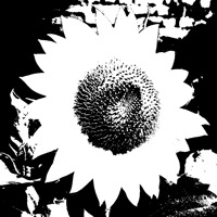
Example: Brightness Threshold
def setup():
    global source, destination
    size(200, 200)
    source = loadImage("sunflower.jpg")
    # The destination image is created as a blank image the same size as the source.
    destination = createImage(source.width, source.height, RGB)

def draw():
    threshold = 127

    # We are going to look at both image's pixels
    source.loadPixels()
    destination.loadPixels()

    for x in xrange(source.width):
        for y in xrange(source.height):
            loc = x + y*source.width
            # Test the brightness against the threshold
            if (brightness(source.pixels[loc]) > threshold):
                destination.pixels[loc]  = color(255) # White
            else:
                destination.pixels[loc]  = color(0)   # Black


    # We changed the pixels in destination
    destination.updatePixels()
    # Display the destination
    image(destination,0,0)
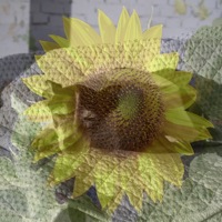
// Draw the image
image(img,0,0)
# Filter the window with a threshold effect
# 0.5 means threshold is 50% brightness
filter(THRESHOLD,0.5)
Level II: Pixel Group Processing
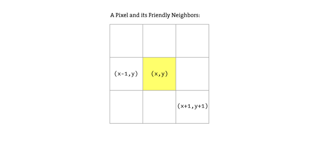
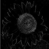
In previous examples, we've seen a one-to-one relationship between source pixels and destination pixels. To increase an image's brightness, we take one pixel from the source image, increase the RGB values, and display one pixel in the output window. In order to perform more advanced image processing functions, we must move beyond the one-to-one pixel paradigm into pixel group processing.
loc = x + y*img.width
pix = img.pixels[loc]
leftLoc = (x-1) + y*img.width
leftPix = img.pixels[leftLoc]
diff = abs(brightness(pix) - brightness(leftPix))
pixels[loc] = color(diff)
# Since we are looking at left neighbors
# We skip the first column
for x in xrange(width):
    for y in xrange(height):
        # Pixel location and color
        loc = x + y*img.width
        pix = img.pixels[loc]

        # Pixel to the left location and color
        leftLoc = (x-1) + y*img.width
        leftPix = img.pixels[leftLoc]

        # New color is difference between pixel and left neighbor
        diff = abs(brightness(pix) - brightness(leftPix))
        pixels[loc] = color(diff)
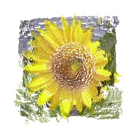
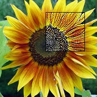
Sharpen:
-1   -1   -1
-1    9   -1
-1   -1   -1

Blur:
1/9  1/9  1/9
1/9  1/9  1/9
1/9  1/9  1/9
w = 80

# It's possible to perform a convolution
# the image with different matrices

matrix =  [ [ -1, -1, -1 ],
            [ -1,  9, -1 ],
            [ -1, -1, -1 ] ]

def setup():
    global img
    size(200, 200)
    frameRate(30)
    img = loadImage("sunflower.jpg")

def draw():
    # We're only going to process a portion of the image
    # so let's set the whole image as the background first
    image(img,0,0)
    # Where is the small rectangle we will process
    xstart = constrain(mouseX-w/2,0,img.width)
    ystart = constrain(mouseY-w/2,0,img.height)
    xend = constrain(mouseX+w/2,0,img.width)
    yend = constrain(mouseY+w/2,0,img.height)
    matrixsize = 3
    loadPixels()
    # Begin our loop for every pixel
    for x in xrange(xstart,xend):
        for y in xrange(ystart,yend):
            # Each pixel location (x,y) gets passed into a function called convolution()
            # which returns a new color value to be displayed.
            c = convolution(x,y,matrix,matrixsize,img)
            loc = x + y*img.width
            pixels[loc] = c

    updatePixels()

    stroke(0)
    noFill()
    rect(xstart,ystart,w,w)

def convolution(x, y, matrix, matrixsize, img):
    rtotal = 0.0
    gtotal = 0.0
    btotal = 0.0
    offset = matrixsize / 2
    # Loop through convolution matrix
    for i in xrange(matrixsize):
        for j in xrange(matrixsize):
            # What pixel are we testing
            xloc = x+i-offset
            yloc = y+j-offset
            loc = xloc + img.width*yloc
            # Make sure we have not walked off the edge of the pixel array
            loc = constrain(loc,0,len(img.pixels)-1)
            # Calculate the convolution
            # We sum all the neighboring pixels multiplied by the convolution matrix values.
            rtotal += (red(img.pixels[loc]) * matrix[i][j])
            gtotal += (green(img.pixels[loc]) * matrix[i][j])
            btotal += (blue(img.pixels[loc]) * matrix[i][j])

    # Make sure RGB is within range
    rtotal = constrain(rtotal,0,255)
    gtotal = constrain(gtotal,0,255)
    btotal = constrain(btotal,0,255)
    # Return the resulting color
    return color(rtotal,gtotal,btotal)
Visualizing the Image
You may be thinking: "Gosh, this is all very interesting, but seriously, when I want to blur an image or change its brightness, do I really need to write code? I mean, can't I use Photoshop?" Indeed, what we have achieved here is an merely an introductory understanding of what highly skilled programmers at Adobe do. The power of Processing, however, is the potential for real-time, interactive graphics applications. There is no need for us to live within the confines of "pixel point" and "pixel group" processing.
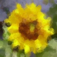
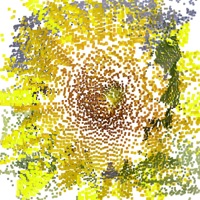
Example: "Pointillism"
pointillize = 16

def setup():
    global img
    size(200,200)
    img = loadImage("sunflower.jpg")
    background(0)
    smooth()

def draw():
    global img, pointillize

    # Pick a random point
    x = int(random(img.width))
    y = int(random(img.height))
    loc = x + y*img.width

    # Look up the RGB color in the source image
    loadPixels()
    r = red(img.pixels[loc])
    g = green(img.pixels[loc])
    b = blue(img.pixels[loc])
    noStroke()

    # Draw an ellipse at that location with that color
    fill(r,g,b,100)
    ellipse(x,y,pointillize,pointillize)
Example: 2D image mapped to 3D
cellsize = 2 # Dimensions of each cell in the grid

def setup():
    global img, cols, rows, cellsize
    size(200, 200, P3D)
    img  = loadImage("sunflower.jpg")  # Load the source image
    cols = width/cellsize              # Calculate number of columns
    rows = height/cellsize             # Calculate number of rows

def draw():
    global img, cols, rows, cellsize

    background(0)
    loadPixels()
    # Begin loop for columns
    for i in xrange(cols):
        # Begin loop for rows
        for j in range(rows):
            x = i*cellsize + cellsize/2  # x position
            y = j*cellsize + cellsize/2  # y position
            loc = x + y*width            # Pixel array location
            c = img.pixels[loc]          # Grab the color
            # Calculate a z position as a function of mouseX and pixel brightness
            z = (mouseX/(float(width))) * brightness(img.pixels[loc]) - 100.0
            # Translate to the location, set fill and stroke, and draw the rect
            pushMatrix()
            translate(x,y,z)
            fill(c)
            noStroke()
            rectMode(CENTER)
            rect(0,0,cellsize,cellsize)
            popMatrix()
This tutorial is for Python Mode of Processing version 2+. If you see any errors or have comments, please let us know. This tutorial is from the book, Learning Processing, by Daniel Shiffman, published by Morgan Kaufmann Publishers, Copyright © 2008 Elsevier Inc. All rights reserved. |

This work is licensed under a Creative Commons Attribution-NonCommercial-ShareAlike 4.0 International License